Major Activities
This work has been completed during this year and is under rereview in International Journal of Computational Fluid Dynamics [paper]. The abtract: Real-time accurate solutions of large-scale complex dynamical systems are in critical need for control, optimization, uncertainty quantification, and decision-making in practical engineering and science applications. This paper contributes in this direction a model-constrained tangent slope learning (mcTangent) approach. At the heart of mcTangent is the synergy of several desirable strategies: i) a tangent slope learning to take advantage of the neural network speed and the time-accurate nature of the method of lines; ii) a model-constrained approach to encode the neural network tangent with the underlying governing equations; iii) sequential learning strategies to promote long-time stability and accuracy; and iv) data randomization approach to implicitly enforce the smoothness of the neural network tangent and its likeliness to the truth tangent up second order derivatives in order to further enhance the stability and accuracy of mcTangent solutions. Both semiheuristic and rigorous arguments are provided to analyze and justify the proposed approach. Several numerical results for transport equation, viscous Burger’s equation, and Navier-Stokes equation are presented to study and demonstrate the capability of the proposed mcTangent learning approach.
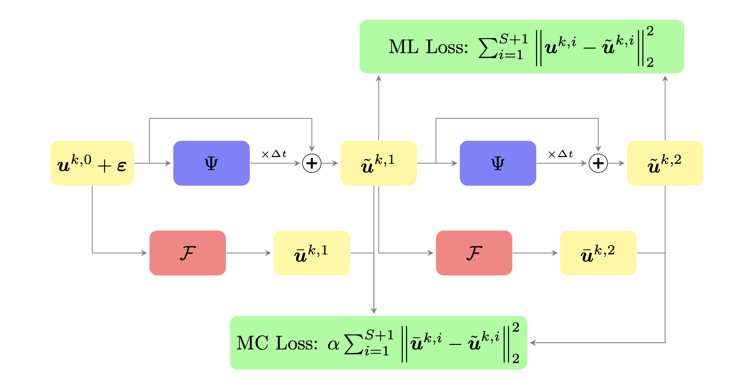 Figure 1: The schematic of mcTangent network architecture for S = 1.
Significant Results
 Figure 2: Wave/transport equation. Trained model-constrained linear neural network weight matrices with model-constrained regularization α = 1e5, noise level δ = 1%. S is number of sequential training steps, R is number of sequential model-constrained steps. The model-constrained weight matrices, after ignoring small elements, have the same structure as the first-order upwind scheme matrix.
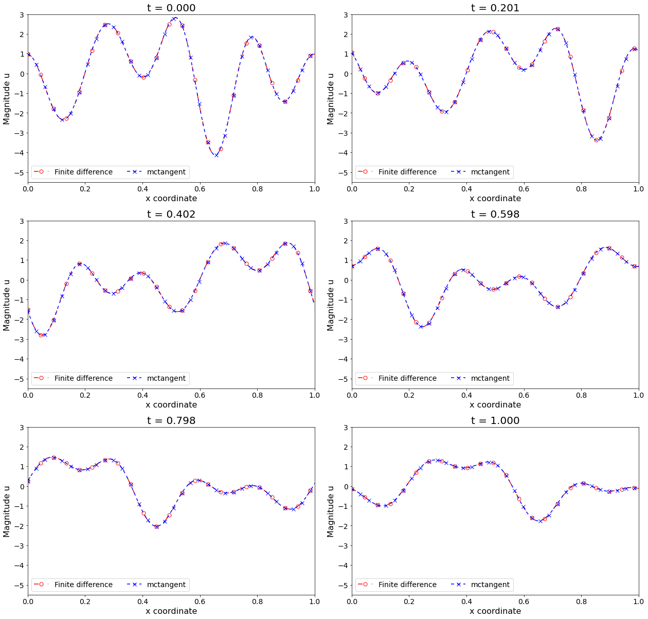 Figure 3: Wave/transport equation. The solutions of Transport/Wave equation obtained by Finite different method versus mcTangent learning approach. Traning data: [0, 0.05], Testing: [0, 1]
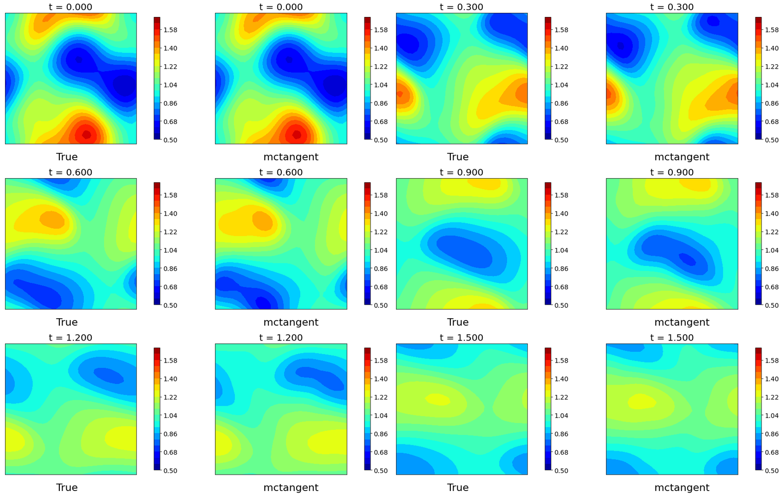 Figure 4: : Burger’s equations. The solutions of Burgers equation obtained by Finite different method versus mcTangent learning approach. Traning data: [0, 0.1], Testing: [0, 1.5]
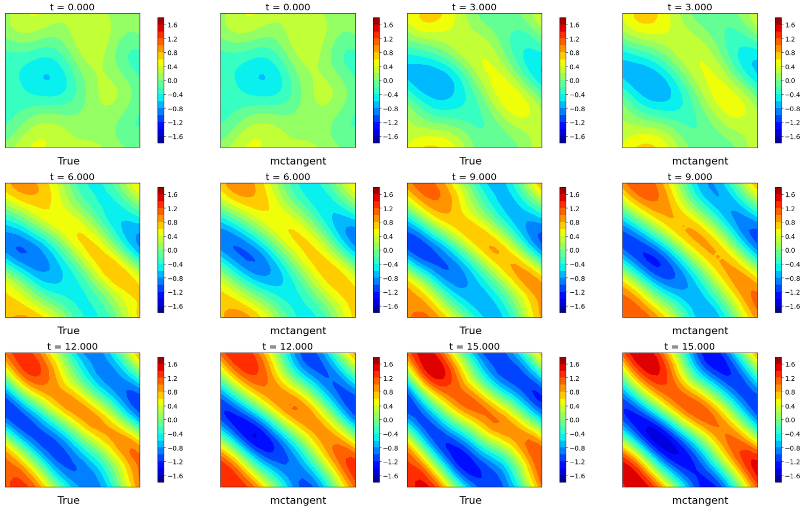 Figure 5: Navier-Stokes equation. The solutions of Navier-Stokes equation obtained by pseudospectra method versus mcTangent learning approach. Traning data: [0, 2], Testing: [0, 15]
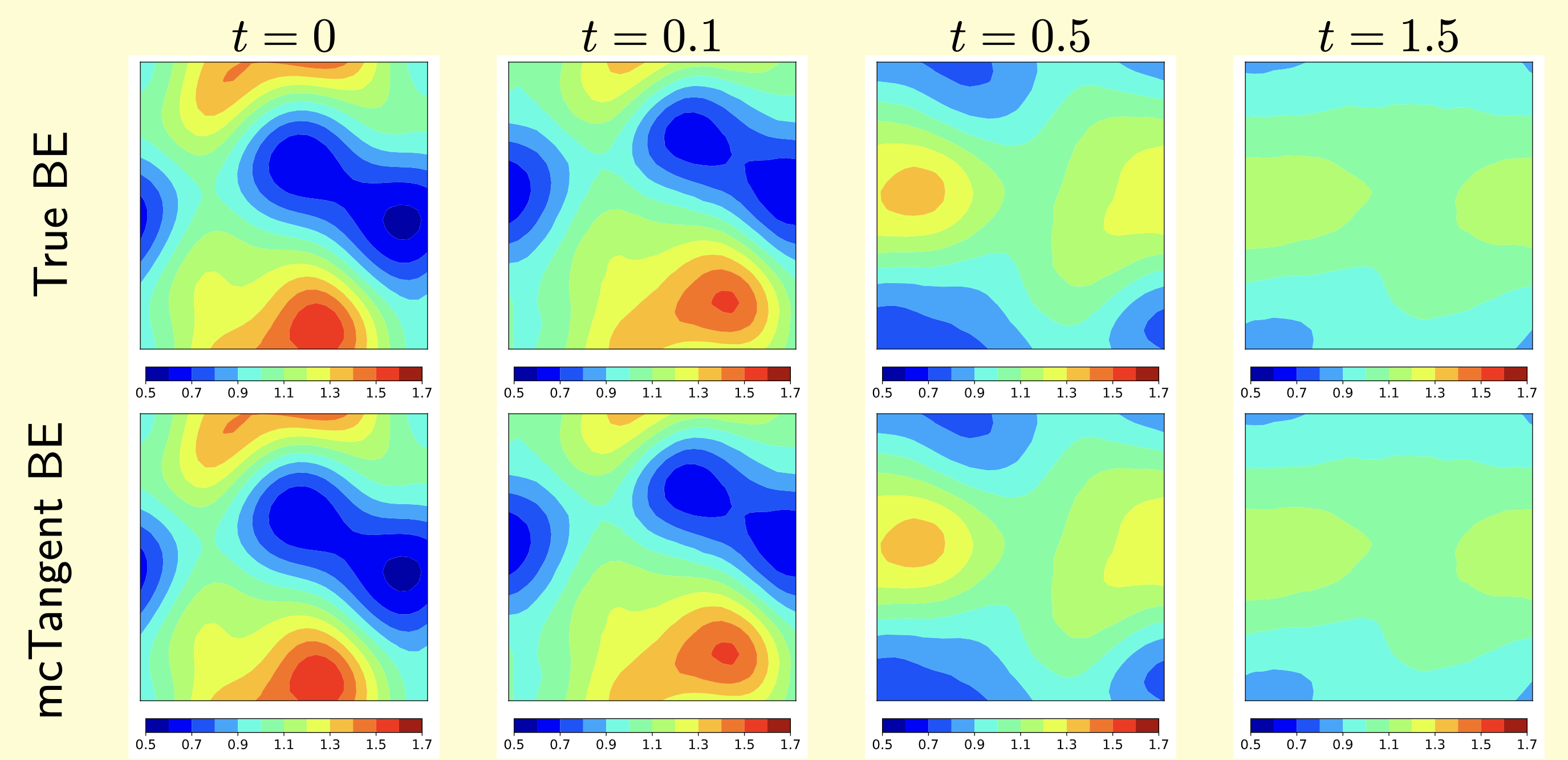 Figure 6: : Burger’s equations. Predicted solutions at different times obtained by Backward Euler (BE) scheme using large stepsize
∆t' = 12.5∆t = 1.25 × 10⁻² with the true tangent slope (True map) and the learned one (Learned map).
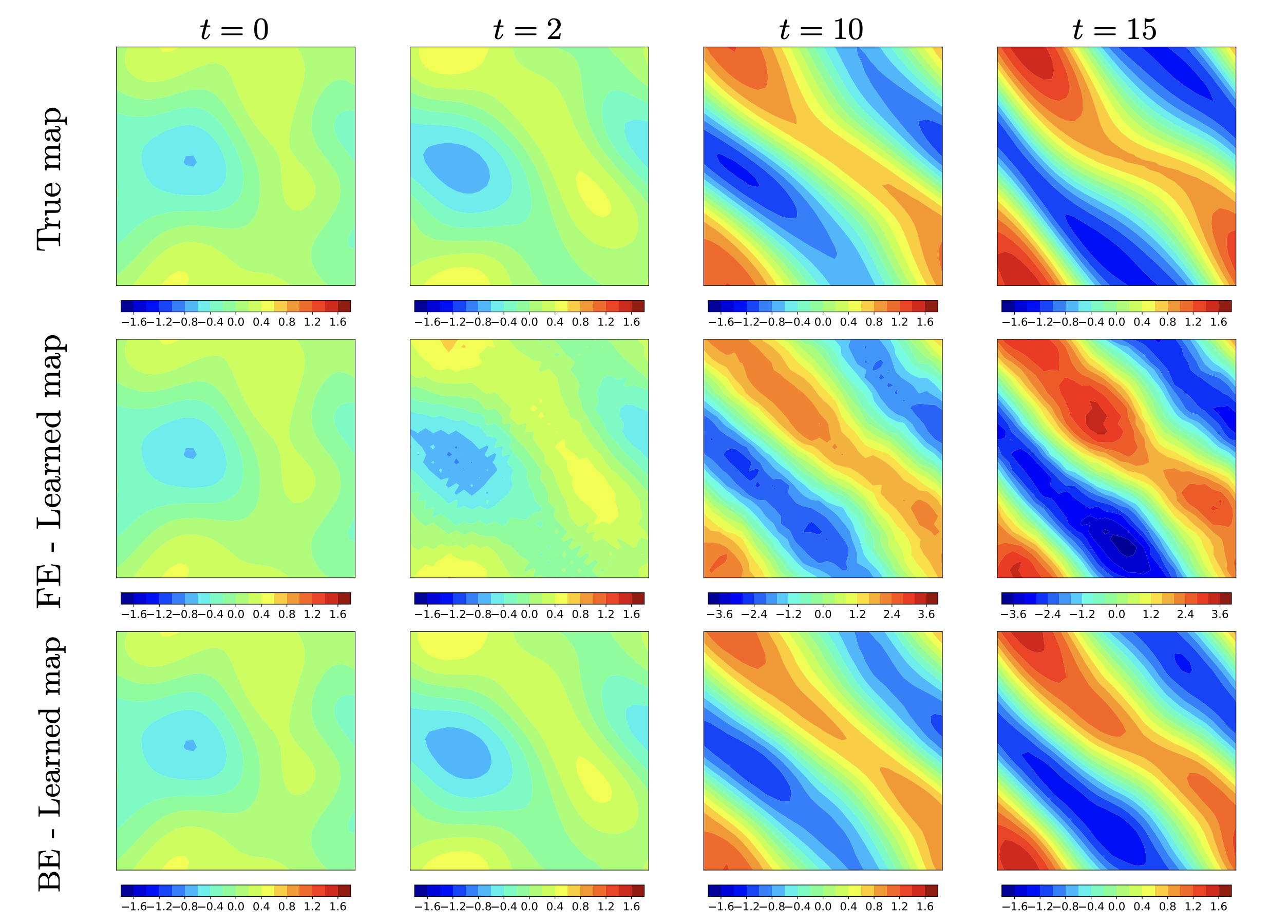 Figure 7: Navier-Stokes equation. Comparison of various neural network solutions. Top row: Spectral method (Crank–Nicolson time integration scheme) with the true tangent slope; Second row: Forward Euler (FE) scheme (a different scale bar in the third and fourth columns); Third row: Backward Euler (BE) scheme with the learned neural network for 20 times larger time stepsize ∆t' = 20∆t.