Active Learning with Neural Architecture Adaptation
Problem description
Last year, we developed and demonstrated two adaptive principles to guide the architecture design of a neural network. In particular, our framework for adaptivity involves computing a quantity called as the “topological derivative” which finds enormous application in the field of structural mechanics, image processing and inverse problems. This year we also explored several potential applications of the “topological derivative” especially in the context of active learning. The problem statement can be summarized as follows:
- Conventional active learning (adaptive data sampling) strategies start by training on a few labeled data samples. In order to confront the overfitting of a small dataset, it is essential to choose a small neural network in the beginning. However, as new data points are queried and added to the training data set, it is essential to increase the capacity of the network to improve the generalization. Therefore, it is essential to develop an active learning framework that incorporates architecture adaptation.
- A well-known issue in statistical active learning literature is the training saturation problem, i.e tendency to get trapped in a local minima and unable to learn on augmenting the training dataset with a new datapoint. It is imperative to have a strategy that handles this issue.
Adopted strategy
In this work we develop a new active learning strategy that incorporates neural network architecture adaptation in the framework. In particular, we provide answers to the following questions:
-
When to add a new layer during the active learning procedure?
-
Where (at which position along the depth) to add a new layer and how to initialize this newly added layer?
-
How does adding a new layer influence the query selection strategy?
-
How to solve the sample saturation and training saturation problem in statistical active learning framework?
Brief outline of the proposed approach
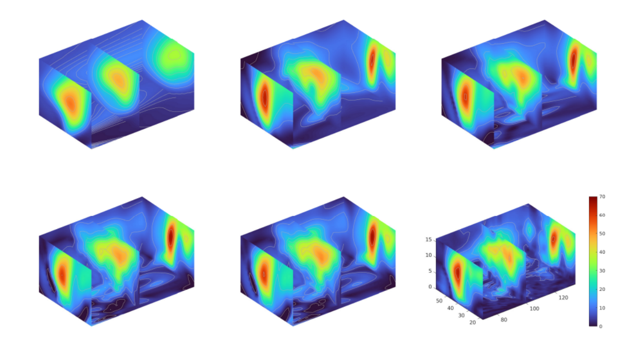
In the active learning procedure, we need to increase the size of the network as more training data-points are available. For this we use employ the topological derivative approach that we developed last year to make a decision on where to add a new layer and how to initialize the new layer. As an example of how the topological derivative approach works, we provide a sample numerical results for a wind velocity reconstruction problem where the objective is to predict the magnitude of wind velocity on a uniform 3D grid based on sparse measurement data. A brief outline of our procedure is as follows: a) Train a small network (with two hidden layers and fixed width) for E epochs; b) Compute the topological derivative for each layer by solving an eigen value problem and identify the optimal location to introduce a new layer along with the corresponding initialization for the parameters; c) Train the new network with the added layer for E epochs; d) Repeat the steps until there is no more improvement in the result (decrease in validation loss). The improvement in solution (3D air current profile) on adding new layers is shown in Figure 1 where one clearly sees that the algorithm progressively picks up complex features in the solution as evident from more contour lines appearing in later stages of the algorithm.
 Figure 1: Evolution of solution (3D air current profile) upon adding new hidden layers (Left to right): Solution after
the 4th iteration; Solution after the 5th iteration; Solution after the 6th iteration; Solution after the 8th iteration;
Solution after the 10th iteration; True solution.
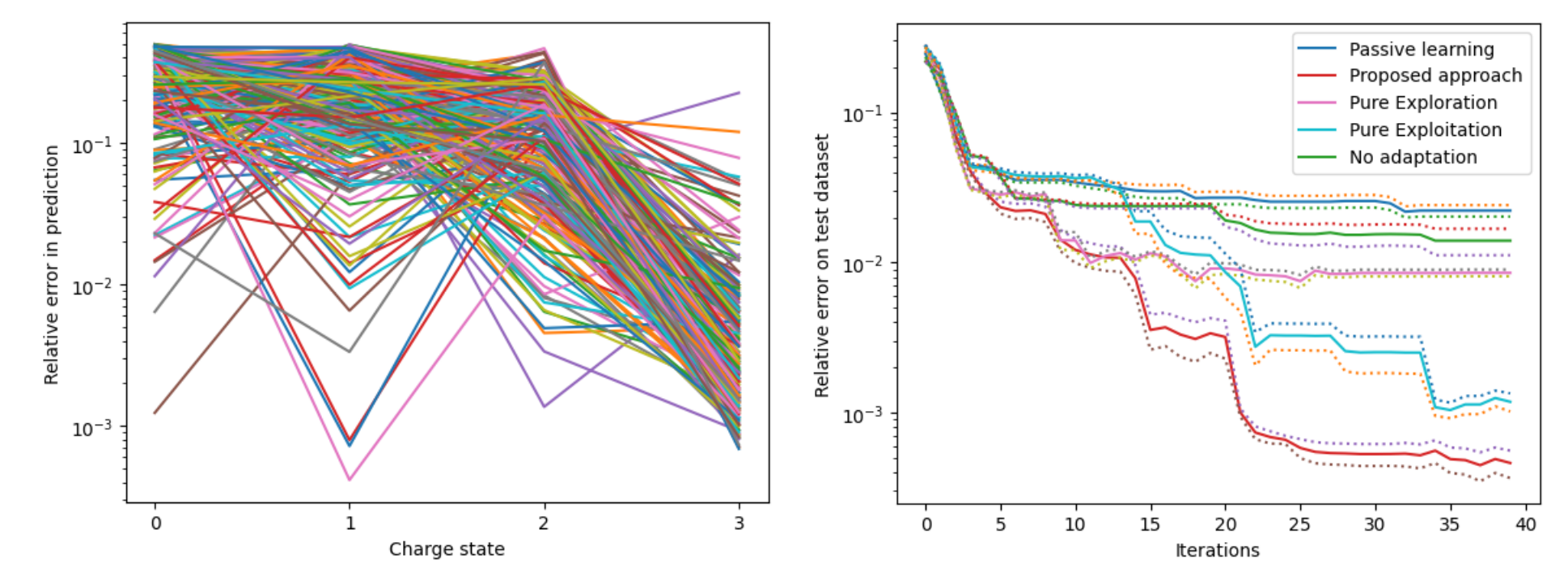
In the context of active learning, our sample selection strategy is based on minimizing the variance of an estimator (neural network) which indirectly improves the generalization (if the bias of the model is small). Note that the variance is a function of the new data-point to be selected. A brief outline of our procedure is as follows: a) Start with a small number of training samples (say 10) and a small network (in our case 2 hidden layer, 20 neurons in each layer with some % sparsity, i.e only a few connections); b) Train the network to some E epochs; c) Add a new data sample by solving an optimization problem; d) Retrain the network and continue the procedure; e) If after adding say r new samples, the validation loss does not decrease, then improve the capacity of the network by adding a new layer with a specific initialization informed by the topological derivative. The procedure is demonstrated on the Collisional-radiative model (CR model) where the objective is to learn the steady state solution for different initial conditions. We start the active learning procedure starting from 10 samples and considered comparing our method with other approaches.
 Figure 2: Left to right: Relative error on the predicted charge state for 250 different test dataset using the proposed
approach (final number of training samples: 50); Comparison between different active learning approaches.
Figure 2 (right) shows that our proposed approach exhibits superior performance in comparison to other active learning strategies. In Figure 2 (right), the term “iterations” refer to each time a new data sample is added to the training data set. Figure 2 (left) shows the point-wise relative error achieved by our proposed framework for the four charge states for 250 different test cases which clearly indicates that our method learns the steady state reasonably well.