Model-constrained Tikhonov Autoencoder Network (TAEN)
Major Activities
The TAEN framework demonstrates remarkable capability in learning both forward and inverse surrogate models from a single observational sample, achieving accuracy on par with traditional Tikhonov regularization solvers. This is a critical breakthrough, as it drastically reduces the dependency on large training datasets, a common bottleneck in conventional machine learning approaches. Central to TAEN’s success is its data randomization strategy, which introduces controlled noise to the input observational data during training. This technique acts as a generative mechanism, effectively exploring the training data space and preventing overfitting—a persistent issue in both purely data-driven and physics-informed neural networks when data is limited. For linear inverse problems, TAEN’s encoder recovers Tikhonov-regularized solutions with precision, ensuring that the learned inverse map adheres to the physical constraints imposed by the governing PDEs. Simultaneously, the decoder accurately represents the forward PtO mapping, achieving exact compliance with the underlying equations at training points. These findings are underpinned by comprehensive theoretical analysis, including forward and inverse inference error bounds, which provide a rigorous justification for TAEN’s performance. The sequential training approach—first optimizing the encoder, then the decoder—further enhances its efficacy, avoiding the convergence difficulties associated with simultaneous encoder-decoder optimization. This combination of minimal data requirements, robust regularization, and theoretical grounding marks TAEN as a highly effective solution for PDE-constrained problems across diverse applications.
Specific Objectives
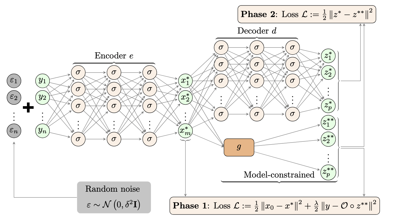
We propose a model-constrained TNet autoencoder approach, termed TAEN. In this framework, the encoder and decoder act as surrogate models for the inverse and forward maps, respectively, as shown in Figure 1. The TAEN network is trained in two phases: phase 1 trains the encoder, and phase 2 trains the decoder using the trained encoder. The total training loss function for TAEN is:
\[\begin{equation} \min \frac{1}{2} \|e(Y) - u_0 1^\top\|_F^2 + \frac{\lambda}{2} \|f(e(Y)) - Y\|_F^2 + \frac{1}{2} \|d(e(Y)) - g(e(Y))\|_F^2, \end{equation}\]where \(e: \mathbb{R}^n \to \mathbb{R}^m\) is the encoder, \(d: \mathbb{R}^m \to \mathbb{R}^p\) is the decoder, \(g: \mathbb{R}^m \to \mathbb{R}^p\) is the PDE solver, \(O: \mathbb{R}^p \to \mathbb{R}^n\) is the observation operator, \(f = O \circ g: \mathbb{R}^m \to \mathbb{R}^n\) is the forward model, \(u_0 \in \mathbb{R}^m\) is the prior mean, \(Y \in \mathbb{R}^{n \times n_t}\) is a matrix of \(n_t\) observation data samples, and \(\|\cdot\|_F\) is the Frobenius norm.
To gain insight into TAEN, we analyze a linear forward problem of the form $y = F u = O \circ G u$ and $z = G u$, using linear encoder and decoder networks, \(z = W_e u + b_e\) and \(u = W_d y + b_d\). We define the mean of observation data \(\bar{y} = Y \frac{1}{n_t}\) and the centered data matrix \(\bar{Y} = Y - \bar{y} 1^\top\). Substituting these into the loss function in (1) and solving analytically yields theoretical results.

Proposition
Suppose \(\bar{Y}\) is full row rank, i.e., \(\bar{Y} \bar{Y}^\dagger = I\), then for a new test pair \((u^\text{test}, y^\text{obs})\), the optimal encoder inverse solution is:
\[u^{\text{TAEN}} = (I + \lambda F^\top F)^{-1} (u_0 + \lambda F^\top \bar{Y} \bar{Y}^\dagger y^\text{obs} + \lambda F^\top (I - \bar{Y} \bar{Y}^\dagger) \bar{y}),\]and the corresponding error is:
\[\|u^{\text{TAEN}} - u^\text{test}\|_2 \le \|u_0 - u^\text{test}\|_2.\]Furthermore, the encoder inverse solution matches the linear Tikhonov regularization problem:
\[\min_u \frac{1}{2} \|u - u_0\|_2^2 + \frac{\lambda}{2} \|F u - y^\text{obs}\|_2^2,\]and the decoder forward solution is exact, i.e., \(z^{\text{TAEN}} = W_d u^\text{test} = G u^\text{test} = z^\text{True}\).
The inverse solution of TAEN is interpretable as a Tikhonov inverse solver for the linear case, with error no larger than the difference between the prior mean and ground truth. The forward decoder solution is exact as \(W_d = G\). Full row rank \(\bar{Y}\) can be achieved from a single sample using data randomization techniques.
Significant Results
Solving forward and inverse problems with 2D Navier-Stokes equations
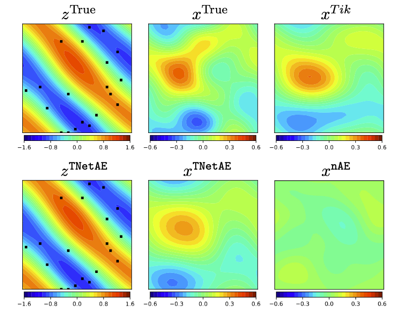
We applied nAE (naive data-driven autoencoder) and TAEN to the Navier-Stokes equation problem, training with one sample. Over 500 test samples, TAEN achieved a 25.68% inverse relative error, comparable to 22.71% by Tikhonov regularization, while nAE yielded 104%. Forward relative errors were 560% for nAE and 0.2% for TAEN.
The three subfigures on the first row of Figure 2 shows ground truth vorticity at \(T = 10s\), initial vorticity, and Tikhonov solution for initial vorticity via PDE-constrained optimization. The second row shows final time vorticity from TAEN, TAEN initial vorticity, and nAE vorticity. TAEN and nAE provide real-time solutions, ~1,240 times faster for forward Navier-Stokes and ~25,000 times faster for inferring initial vorticity from final time observations (black dots).

More detail about this work can be found at https://arxiv.org/abs/2412.07010.