Year 4 - Autoencoder Compression to Accelerate Inverse Problems
Algorithm improvements
We previously proposed an autoencoder based compression approach to eliminate the need for checkpointing in solving time-dependent PDE based inverse problems. We showed the viability of this method on a model acoustic-elastic wave propagation problem on a box-shaped domain, inverting for a deviation from the prior mean acoustic wave speed. This approach wase based on using the Tensorflow SavedModel API where Tensorflow models were trained in Python and loaded in C++ to interface with a sophisticated discontinuous Galerkin finite element solver. While the approach worked fairly well — an overall speedup of ~10% compared to the checkpointing case using CPUs — the performance gains were rather lack-luster.
This year we propose a new method using a novel sparse-dense model approach. This arose from the observation that about 90% of the parameters of the autoencoder lived in the first encoding layer and last decoding layer — the layers that map from and to the higher dimensional state space. By sparsifying only these layers, we reduced the total number of parameters in the autoencoder model by 80% and reduced the computational cost of using the autoencoder to solve the inverse problem. We found empirically that this reduction in representation power of the autoencoder did not negatively impact accuracy in solving the inverse problem.
Results
Building upon the results from the previous year in which we showed that an autoencoder compression strategy works on an acoustic-elastic inverse problem, we now show scaling results for this approach on the model box problem. All results presented here utilize our novel sparse-dense autoencoder architecture and implementation.
| Degrees of freedom | \(\nabla\) Speedup | \(\mathcal{H}v\) Speedup | Relative error % |
|---|---|---|---|
| 4,096 | 1.06 | 1.20 | 1.7 |
| 32,768 | 1.19 | 1.26 | 0.7 |
| 262,144 | 1.17 | 1.22 | 0.6 |
| 2,097,152 | 1.17 | 1.23 | 0.7 |
| 16,777,216 | 1.22 | 1.27 | 0.4 |
\(\nabla\) speedup is the speedup of the gradient computation compared to the checkpointing case and \(\mathcal{H}v\) speedup is the speedup of each Hessian-vector product. Relative errors reported here are the average relative error over the whole domain. This table shows the scaling of our method to a problem that is 64 times larger than the problems considered last year.
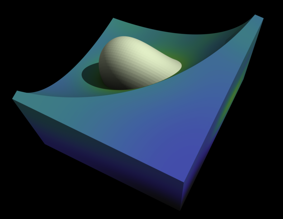
 Inversion result for problem with 16,777,216 degrees of freedom. Shown is an isosurface
of the inclusion in the acoustic wave speed embedded in a cutaway of the domain.
Moving outside of the box
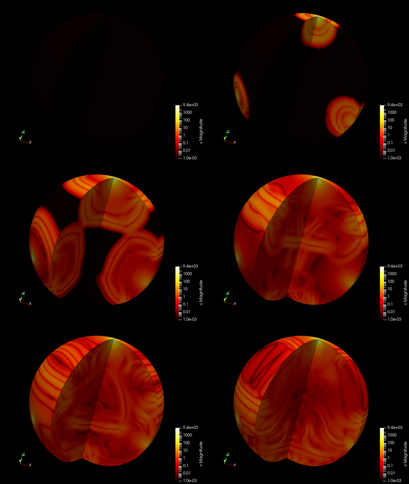
As a capstone example for this project, we are working on implementing our compression approach for an earth-scale seisimic inverse problem. 3 explosion sources are places in the north, southeast, and southwest of North America and an array of 130 seismic sensors throughout the continent record local velocities at each timestep. This setup poses a number of additional challenges that have not been faced in the box example:
- More degrees of freedom
- Adaptive mesh refinement
- Non-conforming mesh with hanging faces
- Non-uniform per-process work distribution We are actively working on adapting our compression strategy to this new challenging setup.
 Shown here is an animation of the velocity timeseries created from the 3 source setup.

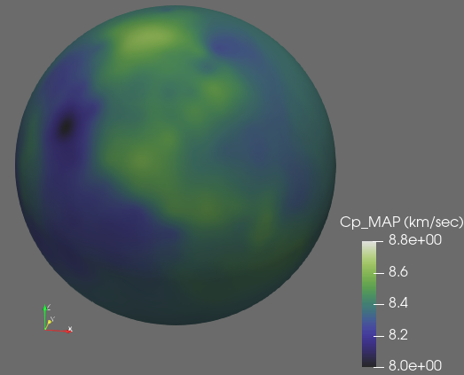
We aim to invert for the wave speed throughout the earth, but in particular aim to accurately recover the properties of the North American continent. The checkpointing strategy yields the inversion results shown above. Results using the autoencoder compression strategy are expected in the next month, at which point we will submit the work for publication.