TAEN: A Model-Constrained Tikhonov Autoencoder Network for Forward and Inverse Problems

Paper publication

Publication Link: https://www.sciencedirect.com/science/article/abs/pii/S0045782525005171

Citation:

@article{van2025taen,
  title={TAEN: a model-constrained Tikhonov autoencoder network for forward and inverse problems},
  author={Van Nguyen, Hai and Bui-Thanh, Tan and Dawson, Clint},
  journal={Computer Methods in Applied Mechanics and Engineering},
  volume={446},
  pages={118245},
  year={2025},
  publisher={Elsevier}
}

---

Table of Contents

• Paper publication
• Table of Contents
• Objectives
• Significant Results
  • Methodology
  • Problem 1: 2D Heat Equation
  • Problem 2: 2D Navier-Stokes Equations
  • Training Cost and Speedup with Deep Learning Solutions

---

Objectives

Efficient real-time solvers for forward and inverse problems are essential in engineering and science applications. Machine learning surrogate models have emerged as promising alternatives to traditional methods, offering substantially reduced computational time. Nevertheless, these models typically demand extensive training datasets to achieve robust generalization across diverse scenarios. While physics-based approaches can partially mitigate this data dependency and ensure physics-interpretable solutions, addressing scarce data regimes remains a challenge. Both purely data-driven and physics-based machine learning approaches demonstrate severe overfitting issues when trained with insufficient data.

We propose a novel model-constrained Tikhonov autoencoder neural network framework, called TAEN, capable of learning both forward and inverse surrogate models using a single arbitrary observational sample. We develop comprehensive theoretical foundations including forward and inverse inference error bounds for the proposed approach for linear cases. For comparative analysis, we derive equivalent formulations for pure data-driven and model-constrained approach counterparts. At the heart of our approach is a data randomization strategy with theoretical justification, which functions as a generative mechanism for exploring the training data space, enabling effective training of both forward and inverse surrogate models even with a single observation, while regularizing the learning process. We validate our approach through extensive numerical experiments on two challenging inverse problems: 2D heat conductivity inversion and initial condition reconstruction for time-dependent 2D Navier-Stokes equations. Results demonstrate that TAEN achieves accuracy comparable to traditional Tikhonov solvers and numerical forward solvers for both inverse and forward problems, respectively, while delivering orders of magnitude computational speedups.

Significant Results

Methodology

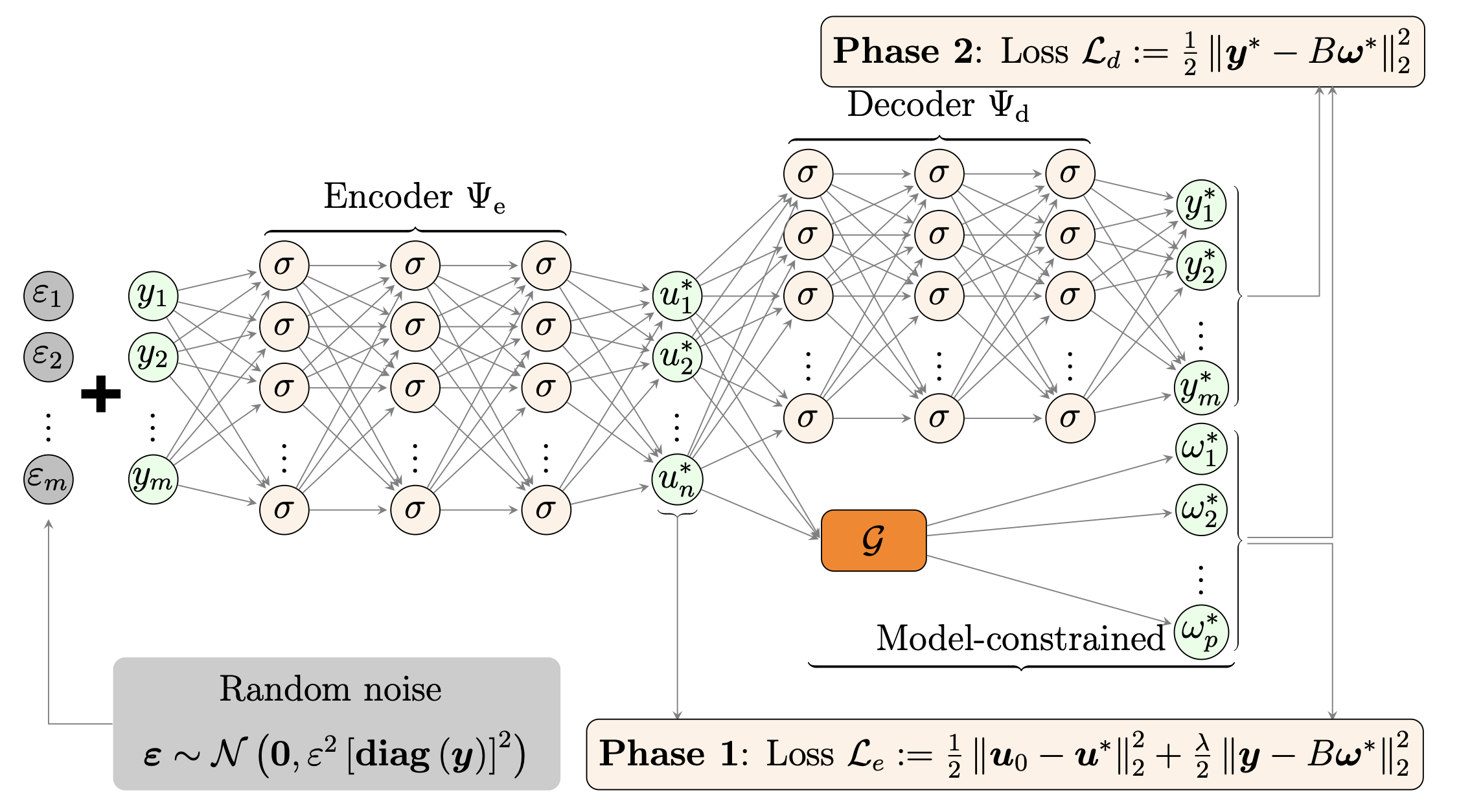
The TAEN framework employs a model-constrained autoencoder architecture that learns both forward and inverse mappings simultaneously. The key innovation is the integration of Tikhonov regularization principles with data randomization techniques and using the physics model to constrain the neural networks, enabling effective learning from minimal training data.

Figure 1: The schematic of TAEN approach. A sequential learning strategy is applied to learn the encoder and decoder in two phases. In Phase 1, at every epoch during training, we randomize the observation data with noise \(\boldsymbol{\epsilon} \sim \mathcal{N}(0, \epsilon^2 [\text{diag}(\mathbf{y})]^2)\) which is added to the observation data \(\mathbf{y}\) to generate randomized observation samples. The randomized data is then fed into the encoder network \(\Psi_e\) to predict the inverse solution \(\mathbf{u}^*\). The predicted inverse \(\mathbf{u}^*\) is passed to the PtO map \(\mathbf{B} \circ \mathcal{F}\) to predict the observation data \(\mathbf{B}\mathbf{y}_{\text{full}}^{*}\). The regularization parameter \(\lambda\) is to balance loss terms. We minimize the encoder loss \(\mathcal{L}_e\) for the optimal encoder network. In Phase 2, we randomize observations and pass through the pre-trained encoder network to produce inverse solutions \(\mathbf{u}^*\). Then, \(\mathbf{u}^*\) is treated as inputs to both the decoder network \(\Psi_d\) to produce \(\mathbf{y}^*\) and PtO map to produce \(B\boldsymbol{\omega}^*\). The decoder loss \(\mathcal{L}_d\) is then minimized to find optimal decoder parameters.

Loss Functions for Different Approaches:

We compare several autoencoder approaches for learning forward and inverse mappings. Here are the key loss functions:

1. Pure POP (Purely data-driven Parameter-to-Observable-to-Parameter):
   • Encoder: \(\min \frac{1}{2} \|\Psi_e(\mathbf{P}) - \mathbf{Y}\|_F^2\)
   • Decoder: \(\min \frac{1}{2} \|\Psi_d(\Psi_e^*(\mathbf{P})) - \mathbf{P}\|_F^2\)
2. Pure OPO (Purely data-driven Observable-to-Parameter-to-Observable):
   • Encoder: \(\min \frac{1}{2} \|\Psi_e(\mathbf{Y}) - \mathbf{P}\|_F^2\)
   • Decoder: \(\min \frac{1}{2} \|\Psi_d(\Psi_e^*(\mathbf{Y})) - \mathbf{Y}\|_F^2\)
3. mcPOP (Model-constrained Parameter-to-Observable-to-Parameter):
   • Encoder: \(\min \frac{1}{2} \|\Psi_e(\mathbf{P}) - \mathbf{Y}\|_F^2\)
   • Decoder: \(\min \frac{1}{2} \|\Psi_d(\Psi_e^*(\mathbf{P})) - \mathbf{P}\|_F^2 + \frac{\lambda}{2} \|\mathbf{B} \circ \mathcal{F}(\Psi_d(\Psi_e^*(\mathbf{P}))) - \mathbf{Y}\|_F^2\)
4. mcOPO (Model-constrained Observable-to-Parameter-to-Observable):
   • Encoder: \(\min \frac{1}{2} \|\Psi_e(\mathbf{Y}) - \mathbf{U}\|_F^2 + \frac{\lambda}{2} \|\mathbf{B} \circ \mathcal{F}(\Psi_e(\mathbf{Y})) - \mathbf{Y}\|_F^2\)
   • Decoder: \(\min \frac{1}{2} \|\Psi_d(\Psi_e^*(\mathbf{Y})) - \mathbf{B} \circ \mathcal{F}(\Psi_e^*(\mathbf{Y}))\|_F^2\)
5. mcOPOfull (Model-constrained Observable-to-Parameter-to-Forward):
   • Encoder: \(\min \frac{1}{2} \|\mathbf{U} - \Psi_e(\mathbf{Y})\|_F^2 + \frac{\lambda}{2} \|\mathbf{Y} - \mathbf{B} \circ \mathcal{F}(\Psi_e(\mathbf{Y}))\|_F^2\)
   • Decoder: \(\min \frac{1}{2} \|\mathcal{F}(\Psi_e^*(\mathbf{Y})) - \Psi_d(\Psi_e^*(\mathbf{Y}))\|_F^2\)
6. TAEN (Tikhonov Autoencoder Network):
   • Encoder: \(\min \frac{1}{2} \|\Psi_e(\mathbf{Y}) - \mathbf{u}_0 \mathbf{1}^T\|_F^2 + \frac{\lambda}{2} \|\mathbf{B} \circ \mathcal{F}(\Psi_e(\mathbf{Y})) - \mathbf{Y}\|_F^2\)
   • Decoder: \(\min \frac{1}{2} \|\Psi_d(\Psi_e^*(\mathbf{Y})) - \mathbf{B} \circ \mathcal{F}(\Psi_e^*(\mathbf{Y}))\|_F^2\)
7. TAENfull (Tikhonov Autoencoder Network - Full Forward Map):
   • Encoder: \(\min \frac{1}{2} \|\Psi_e(\mathbf{Y}) - \mathbf{u}_0 \mathbf{1}^T\|_F^2 + \frac{\lambda}{2} \|\mathbf{B} \circ \mathcal{F}(\Psi_e(\mathbf{Y})) - \mathbf{Y}\|_F^2\)
   • Decoder: \(\min \frac{1}{2} \|\mathcal{F}(\Psi_e^*(\mathbf{Y})) - \Psi_d(\Psi_e^*(\mathbf{Y}))\|_F^2\)

where \(\Psi_e\) and \(\Psi_d\) are encoder and decoder networks, \(\mathbf{P}\) and \(\mathbf{Y}\) are training parameter and observation data, \(\mathcal{F}\) is the forward model (PDE solver), \(\mathbf{B}\) is the observation operator, \(\lambda\) is the regularization parameter, and \(\mathbf{u}_0\) is the prior mean of parameters. The key difference of TAEN is that it uses \(\mathbf{u}_0\) instead of ground truth parameters \(\mathbf{P}\), enabling learning from a single observation sample.

Problem 1: 2D Heat Equation

We investigate the following heat equation:

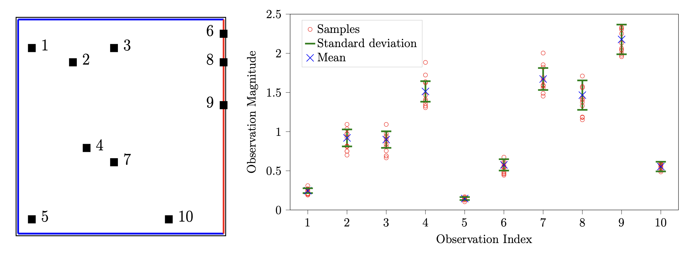
\[\begin{align*} -\nabla \cdot (e^u \nabla \omega) & = 20 \quad \text{in } \Omega = (0,1)^2 \\ \omega & = 0 \quad \text{ on } \Gamma^{\text{ext}} \\ \textbf{n} \cdot (e^u \nabla \omega) & = 0 \quad \text{ on } \Gamma^{\text{root}}, \end{align*}\]

where \(u\) represents the (log) conductivity coefficient field (the parameter of interest PoI), \(\omega\) denotes the temperature field, and \(\textbf{n}\) is the unit outward normal vector along the Neumann boundary \(\Gamma^{\text{root}}\). As illustrated in the left panel of Figure 2, we discretize the domain using a \(16 \times 16\) grid, with 10 randomly distributed observation points sampling from the discretized field \(\mathbf{y}_{\text{full}}\).

We aim to achieve two primary goals: (1) learning an inverse mapping to directly reconstruct the conductivity coefficient field \(\mathbf{u}\) from 10 discrete observations \(\mathbf{y} = \mathbf{B} \mathbf{y}_{\text{full}}\), and (2) learning a PtO map or forward map that predicts either the temperature observations \(\mathbf{y}\) or the temperature field \(\mathbf{y}_{\text{full}}\) given a conductivity coefficient field \(\mathbf{u}\).

Figure 2: 2D heat equation. Left: A sample of the PoI (the heat conductivity field). Right: The corresponding state (temperature field), observations (temperatures) are taken at 10 observed points. This pair of PoI and observation sample is used for training in one training sample case. The middle and right figures show the conductivity coefficient fields \(u\) and its corresponding temperature field \(\mathbf{y}_{\text{full}}\) for the first pair out of 100 training sample pairs. This particular pair serves as the training data for the single-sample training case for all approaches.

The following table summarizes the average relative error for inverse solutions and forward solutions (observations) over 500 test samples obtained by all approaches trained with {1,100} training samples. The model-constrained approaches are more accurate for both inverse (comparable to the Tikhonov—Tik—approach) and forward solution, and within the model-constrained approaches, TAEN and TAENfull are the most accurate ones: in fact one training sample is sufficient for these two methods.

Approach	Inverse (%) (1 sample)	Forward (1 sample)	Inverse (%) (100 samples)	Forward (100 samples)
Pure POP	100.18	3.99×10⁻¹	80.48	5.30×10⁻²
Pure OPO	107.55	2.90×10⁻¹	50.18	1.09×10⁻¹
mcPOP	107.99	3.99×10⁻¹	87.60	5.30×10⁻²
mcOPO	108.28	2.73×10⁻²	46.32	3.94×10⁻⁴
mcOPOfull	108.28	4.21×10⁻²	46.32	4.56×10⁻⁴
TAEN	45.23	1.57×10⁻⁴	45.03	1.22×10⁻⁴
TAENfull	45.23	8.80×10⁻⁴	45.03	2.12×10⁻⁴
Tikhonov	44.99	-	44.99	-

Table 1: 2D heat equation. The average relative error for inverse solutions and forward solutions (observations) over 500 test samples obtained by all approaches trained with {1,100} training samples. The model-constrained approaches are more accurate for both inverse (comparable to the Tikhonov—Tik—approach) and forward solution, and within the model-constrained approaches, TAEN and TAENfull are the most accurate ones: in fact one training sample is sufficient for these two methods. We compare all approaches using the aforementioned two-phase sequential training protocol. All methods are implemented under two scenarios: training with a single training sample and training with 100 training samples. For mcOPO, mcOPOfull, TAEN, and TAENfull approaches, we perform data randomization for each epoch by adding random noise with magnitude \(\epsilon = 10\%\) to the already-noise-corrupted observation samples.

Generating train and test data sets.

We start with drawing the parameter conductivity samples via a truncated Karhunen-Loève expansion

\[u(x) = \sum_{i =1 }^q \sqrt{\lambda_i} \boldsymbol{\phi}_i(x) \mathbf{u}_i, \quad x \in [0,1]^2,\]

where \((\lambda_i, \boldsymbol{\phi}_i)\) is the eigenpair of a two-point correlation function, and \(\mathbf{u} = \{\mathbf{u}_i\}_{i=1}^q \sim \mathcal{N}(0,\mathbf{I})\) is a standard Gaussian random vector. We choose \(q = 15\) eigenvectors corresponding to the first \(15\) largest eigenvalues. For each sample \(\mathbf{u}\), we solve the heat equation for the corresponding temperature field \(\mathbf{y}_{\text{full}}\) by the finite element method. The observation samples \(\mathbf{y}^{\text{clean}}\) are constructed by extracting values of the temperature field \(\mathbf{y}_{\text{full}}\) at the 10 observable locations, followed by the addition of Gaussian noise with the noise level of \(\delta = 0.5\%\). Our training dataset consists of 100 independently drawn sample pairs. For the inference (testing) step, we generate 500 independently drawn pairs \((\mathbf{u}, \mathbf{y}_{\text{full}})\) following the same procedure discussed above.

Learned inverse and PtO/forward maps accuracy.

Approach	1 training sample mean	1 training sample std	100 training samples mean	100 training samples std
Pure POP
Pure OPO
mcPOP
mcOPO / mcOPOfull
TAEN / TAENfull
Tik

Figure 3: 2D heat equation. Mean and standard deviation of absolute error for 500 test inverse solutions obtained from different approaches. Black points are observational locations. Note that TAEN and TAENfull (and similarly for Pure POP and mcPOP approaches) have the same encoder (that encodes the inverse solutions), their (identical) results are shown on the 5th row. Relative to the Tikhonov approach (Tik), the model-constrained approaches are more accurate, and within the model-constrained approaches, TAEN and TAENfull are the most accurate ones: in fact, one training sample is sufficient for these two methods. TAEN and TAENfull attain inverse solution accuracy of 45.23%, comparable to the traditional Tikhonov regularization method with 44.99% error. In contrast, all other methodologies (Pure POP, Pure OPO, mcPOP, mcOPO, and mcOPOfull) fail to produce meaningful results. This performance disparity is due to the superior generalization capability of the TAEN and TAENfull approaches, while other methods suffer from overfitting the provided training sample. The data randomization technique serves two crucial functions: Exploring the unseen test observation sample space and exploiting the underlying physics via the model-constrained term.

	Pure POP / mcPOP	Pure OPO	mcOPO	mcOPOfull	TAEN	TAENfull
1 sample
100 samples

Figure 4: 2D heat equation. The comparison of 500 test predicted forward solutions (at the observational locations) obtained from different approaches. In all plots, the x-axis is the magnitude of the true observation, and the y-axis is the magnitude of the predicted observation, both axes have a range of \([0,3]\). The red line indicates the perfect match between predictions and true observations. Top row: Trained with \(1\) training sample. Bottom row: Trained with \(100\) training samples. As can be seen, model-constrained approaches are more accurate, and within the model-constrained approaches, TAEN and TAENfull are the most accurate ones: in fact, one training sample is sufficient for these two methods. TAEN and TAENfull can achieve highly accurate predictions of temperature solutions through the PtO/forward map (decoder), achieving relative errors of 1.57e-04 and 8.80e-04, respectively. This demonstrates their capability to learn accurately PtO/forward mappings from a single observation sample, again thanks to the data randomization. Since TAEN learns the observations directly, it is more accurate than TAENfull which aims to learn the full solution state. While our analysis indicates that mcOPO and mcOPOfull can theoretically learn exact PtO/forward maps in linear problems, their actual performance (errors of 2.73e-02 and 4.21e-2, respectively) falls short compared to TAEN and TAENfull. This underperformance can be attributed to two key factors: inaccurate inverse solutions obtained from the encoder and the nonlinear forward map. On the other hand, Pure POP, Pure OPO, and mcPOP yield inaccurate PtO mappings, which is consistent with their purely data-driven architecture that does not encode physical constraints. For the larger data set of 100 samples, the accuracy of forward and inverse maps for all approaches is improved as expected. TAEN and TAENfull maintain their superior performance for both PtO/forward and inverse solutions. We emphasize that the best inverse map obtained from TAEN and TAENfull is just as good as the Tikhonov regularization method; thus, not much improvement is observed compared to the single-sample training case. In other words, one training data is sufficient for TAEN and TAENfull. Coming in second are mcOPO and mcOPOfull. Unlike the single-sample training scenario, these approaches now achieve reliable inverse maps (encoders), enabling their model-constrained decoders to achieve high accuracy in PtO/forward solutions. Meanwhile, the purely data-driven approach Pure OPO, without additional information provided by the physics constraints, produces lower accuracy in inverse solutions compared to mcOPO. This is not surprising, as the inaccurate inverse solutions from its encoder network inevitably lead to poor PtO solutions, resulting in its least accuracy. On the other hand, the Pure POP and mcPOP approaches, which prioritize learning the PtO map (encoder), achieve better PtO solution accuracy than Pure OPO. Consequently, the inaccuracy of encoder outputs (due to the nonlinear PtO map) propagates through the decoder, resulting in the least accurate inverse solutions, even with the forward solver as the physics constraint.

	1 training sample mean	1 training sample std	100 training samples mean	100 training samples std
mcOPOfull
TAENfull

Figure 5: 2D heat equation. Mean and standard deviation of absolute pointwise error for 500 full state test solutions obtained from TAENfull and mcOPOfull. Black dots are the observational locations. The former is more accurate, especially for the case with one training sample, in which it achieves two orders of magnitude smaller error. TAENfull framework demonstrates consistently lower error statistics (two orders of magnitude smaller for one-sample case) compared to mcOPOfull. The spatial distribution of prediction errors is further examined here, which depicts the mean and standard deviation of absolute pointwise errors for 500 test temperature field samples (unseen full state solutions).

$$\mathbf{u}_\text{Tik}$$	$$\mathbf{u}_{\text{TAENfull}}$$	$$\mathbf{u}_\text{True}$$	$$\mathbf{y}_{\text{TAENfull}}$$
$$\|\mathbf{u}_\text{Tik} - \mathbf{u}_\text{True}\|$$	$$\|\mathbf{u}_{\text{TAENfull}} - \mathbf{u}_\text{True}\|$$	$$\mathbf{y}_\text{True}$$	$$\|\mathbf{y}_{\text{TAENfull}} - \mathbf{y}_\text{True}\|$$

Figure 6: 2D heat equation. A (random) representative case of inverse and full forward solution obtained by TAENfull trained with 1 training sample coupled with data randomization of noise level \(\sigma = 0.1\). TAENfull inverse solution is comparable to the Tikhonov (Tik) inverse counterpart, and both are consistent with the ground truth (True). TAENfull full forward solution is almost identical (in fact within 3 digits of accuracy) to the underlying true solution. It can be seen that the inverted conductivity field exhibits accuracy comparable to the Tikhonov regularization solution, and both closely approximate the true conductivity field distribution. Furthermore, the predicted temperature field demonstrates excellent agreement with the ground truth solution. These results underscore the effectiveness of combining model-constrained learning with data randomization techniques in the TAENfull framework. The significant difference in the test case in Figure 6 and the training sample in Figure 2 demonstrates the framework's robust generalization capabilities to completely different test samples. This desirable characteristic enables the development of inverse and forward surrogate models using minimal training data—namely one single training sample without ground truth PoI—while maintaining reliable performance on unseen test cases. We would like to point out that such a capability comes with an offline cost: a differentiable forward solver is required in this paper. One remedy is to train a surrogate (e.g. neural network) for the forward map or to use a differentiable reliable surrogate if available.

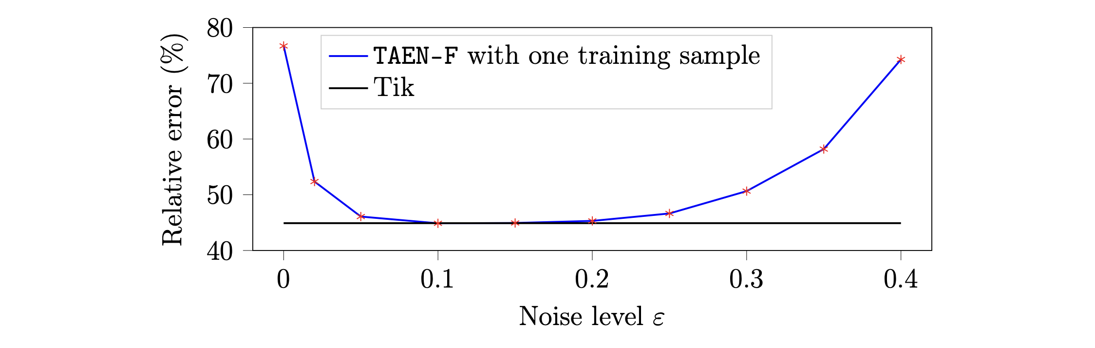
TAENfull robustness to a wide range of noise levels.

We further investigate the robustness of TAENfull across varying noise levels using a single training sample.

Figure 7: 2D heat equation. Relative error of inverse solution over 500 test samples with different noise levels. Figure 7 demonstrates that TAENfull achieves relative errors comparable to the Tikhonov regularization framework across a broad noise spectrum (8% to 20%) for 500 test inverse solutions. Outside this "optimal range", TAENfull does not yield acceptable accuracy. On the one hand, with low noise levels, the data randomization technique insufficiently explores the space of potentially unseen test samples, limiting generalization capabilities. On the other hand, excessive noise levels result in overwhelmingly corrupted samples that are statistically indistinguishable, and thus degrading the accuracy of the learned surrogate models. We would like to point out that the minimum relative error achieved by TAENfull matches that of the Tikhonov regularization framework, indicating that, as designed, TAENfull successfully learns the Tikhonov regularization solver using only a single training sample without requiring ground truth PoI data.

TAENfull robustness to arbitrary single-sample.

In this section, we investigate the robustness of the TAENfull framework to one arbitrarily chosen sample for training. To that end, ten independent training instances are conducted, each utilizing a single sample randomly selected from a pool of 100 training samples.

Figure 8: 2D heat equation. Left: Index of \(10\) observational locations. Right: Mean and standard deviation of observation magnitudes of 10000 true observation samples at the observational locations. The magnitudes of the predicted solutions of 10 different observation samples for single-sample training cases. The left figure in Figure 8 presents the spatial distribution of 10 observational points, including their location indices. The right figure of Figure 8 shows the statistical characteristics (mean and standard deviation) of 10000 distinct observation samples, and the observation magnitudes for the 10 randomly selected training cases at their respective locations. Statistical analysis of the TAENfull performance across these 10 distinct training instances yields an average relative error of 45.32% (again similar to the Tikhonov regularization error) with a standard deviation of 0.32% for inverse solutions. This small variance in relative error metrics demonstrates the TAENfull robustness with respect to an arbitrary individual sample in the single-sample training scenario. In particular, the result shows that the prediction error is similar for any of these 10 individual random samples when used in the TAENfull as the only training sample.

Problem 2: 2D Navier-Stokes Equations

The vorticity form of 2D Navier–Stokes equation for viscous and incompressible fluid is written as

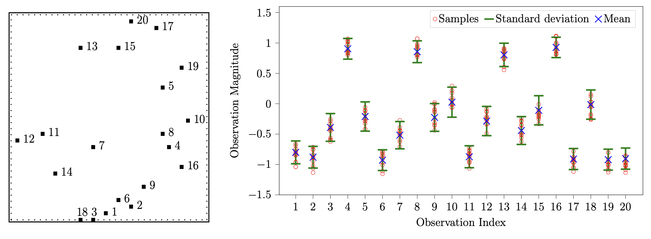
\[\begin{aligned} \partial_t \omega(x,t) + v(x,t) \cdot \nabla \omega(x,t) & = \nu \Delta \omega(x,t) + f(x), & \quad x \in (0,1)^2, t \in (0, T], \\ \nabla \cdot v(x,t) & = 0, & \quad x \in (0,1)^2, t \in (0, T], \\ \omega(x,0) & = u(x), & \quad x \in (0,1)^2, \end{aligned}\]

where \(v \in (0,1)^2 \times (0, T]\) denotes the velocity field, \(\omega = \nabla \times v\) represents the vorticity, and \(u\) defines the initial vorticity which is the parameter of interest. The forcing function is specified as \(f(x) = 0.1 (\sin(2 \pi (x_1 + x_2)) + \cos(2 \pi (x_1 + x_2)))\), with viscosity coefficient \(\nu = 10^{-3}\). The computational domain is discretized using a uniform \(32 \times 32\) mesh in space, while the temporal domain \(t \in (0, 10]\) is partitioned into 1000 uniform time steps with \(\Delta t = 10^{-2}\). The inverse problem aims to reconstruct the initial vorticity field \(u\) from vorticity measurements \(\mathbf{y}\) collected at 20 random spatial locations from the vorticity field \(\omega\) at the final time \(T = 10\).

Figure 9: 2D Navier--Stokes equation. Left: A sample of the PoI \(\mathbf{u}\). Right: A corresponding vorticity field \(\mathbf{y}_{\text{full}}\) at final time \(T = 10\), observation \(\mathbf{y}\) are extracted at 20 random observed points. This pair of PoI and observation/vorticity field is used for training in one training sample case. This figure illustrates the first sample pair from the training dataset of 100 samples, which serves as the training sample for single-sample training scenarios for all approaches.

Approach	Inverse (%) (1 sample)	Forward (1 sample)	Inverse (%) (100 samples)	Forward (100 samples)
Pure POP	156.99	2.99×10⁻¹	72.22	6.72×10⁻²
Pure OPO	103.94	5.60	40.20	5.94×10⁻¹
mcPOP	161.48	2.99×10⁻¹	76.33	6.72×10⁻²
mcOPO	46.43	5.15×10⁻¹	27.29	2.20×10⁻³
mcOPOfull	46.43	3.79×10⁻¹	27.29	2.12×10⁻³
TAEN	25.68	2.14×10⁻³	24.54	1.49×10⁻³
TAENfull	25.68	2.10×10⁻³	24.54	1.45×10⁻³
Tikhonov	22.71	-	22.71	-

Table 2: 2D Navier--Stokes equation. Average relative error for inverse solutions and PtO/forward solutions obtained by all approaches trained with \(\{1,100\}\) training samples. The model-constrained approaches are more accurate for both inverse (comparable to the Tikhonov—Tik—approach) and forward solution, and within the model-constrained approaches, TAEN and TAENfull are the most accurate ones: in fact one training sample is sufficient for these two methods. When trained on a single sample, TAEN and TAENfull achieve the lowest average relative error of 25.68% (closest to the gold-standard Tikhonov regularization solution with 22.71% error) for inverse solutions among all approaches. Similarly, their PtO/forward solutions demonstrate superior accuracy with average relative errors of \(2.14 \times 10^{-3}\) and \(2.10 \times 10^{-3}\), respectively. This generalization accuracy is owing to the combination of data randomization and forward solver model-constrained terms. The mcOPO and mcOPOfull approaches come in second with regard to the accuracy for inverse solutions, with a relative error of 46.43%. This reduced accuracy (relatively to TAEN and TAENfull) stems from a strong bias toward the single training sample, despite the forward solver constraint. mcPOP, Pure OPO, and Pure POP exhibit significantly higher average relative errors of 161.48%, 103.94%, and 156.99% respectively for inverse solutions. These poor results are expected for Pure OPO and Pure POP due to their purely data-driven nature, thus limiting generalization. For mcPOP, the inaccurate encoder (learned PtO map) propagates errors to the decoder training, resulting in imprecise inverse surrogate models. For PtO/forward solutions, Pure POP, Pure OPO, mcPOP, mcOPO, and mcOPOfull fail to produce accurate surrogate models, again due to overfitting to the single training sample despite forward solver regularization. When we increase the number of training samples to 100, and thus providing more information about the problem under consideration, significant accuracy improvements are observed for all approaches for both inverse and PtO/forward surrogate models. TAEN and TAENfull approaches maintain the best performance, achieving average relative errors of 24.54% for inverse solutions compared to the Tikhonov (Tik) method with of 22.71%. Their PtO/forward solutions exhibit good accuracy with average relative errors of \(1.49 \times 10^{-3}\) and \(1.45 \times 10^{-3}\), respectively. The average relative error of the inverse solution obtained by mcOPO and mcOPOfull is \(27.29\%\), which is the second best among all approaches. The relative error of the PtO/forward solution obtained by mcOPO and mcOPOfull is \(2.20 \times 10^{-3}\) and \(2.12 \times 10^{-3}\), respectively, which is almost as good as TAEN and TAENfull. This indicates the roles of model-constrained terms in reducing the overfitting effect when sufficient training data is provided. In contrast, Pure POP and mcPOP show substantially higher relative errors of 72.22% and 76.33%, respectively, for inverse solutions. These high errors stem from inaccuracies in their pre-trained PtO map (encoder), consistent with observations from the single-sample training scenario. Meanwhile, Pure OPO framework shows improved inverse solution accuracy with a relative error of 40.20%, yet remains less accurate than the model-constrained approaches (mcOPO, mcOPOfull, TAEN, and TAENfull). This reduced performance is consistent with the error analysis for linear problems. Moreover, Pure OPO's PtO solution accuracy remains notably poor (\(5.94 \times 10^{-1}\)) despite the richer training dataset with 100 data pairs, reflecting the inherent PtO mapping errors.

Generating train and test data sets.

To generate data pairs of \((u, \omega)\), we draw samples of \(u(x)\) using the truncated Karhunen-Loève expansion

\[u(x) = \sum_{i=1}^{24} \sqrt{\lambda_i} \, \boldsymbol{\phi}_i(x) \, z_i,\]

where \(z_i \sim \mathcal{N}(0, 1), i = 1, \ldots, 24\), and \((\lambda_i, \boldsymbol{\phi}_i)\) are eigenpairs obtained by the eigendecomposition of the covariance operator \(7^{\frac{3}{2}} (-\Delta + 49 \mathbf{I})^{-2.5}\) with periodic boundary conditions. Next, we discretize the initial vorticity \(u(x)\), denoted as \(\mathbf{u}\), and we solve the Navier-Stokes equation by the stream-function formulation with a pseudospectral method to obtain a discrete representation \(\mathbf{y}_{\text{full}}\) of \(\omega(x,t)\) at time \(t = 10\). The observation data \(\mathbf{y}\) consists of the vorticity field \(\mathbf{y}_{\text{full}}\) at \(T = 10\) at 20 randomly distributed observational locations, with the subsequent addition of \(\delta = 2\%\) Gaussian noise. Two distinct datasets are generated: a training set comprising 100 independent samples and a test set containing 500 samples.

Learned inverse and PtO/forward maps accuracy.

Following the same procedure used for the 2D heat equation, encoder and decoder networks are trained sequentially for two cases: using a single training sample pair (shown in Figure 9) and using 100 training sample pairs. For mcOPO, mcOPOfull, TAEN and TAENfull approaches, randomization is performed at each epoch with noise level \(\epsilon = 25\%\).

Approach	1 training sample mean	1 training sample std	100 training samples mean	100 training samples std
Pure POP
Pure OPO
mcPOP
mcOPO / mcOPOfull
TAEN / TAENfull
Tik

Figure 10: 2D Navier--Stokes equation. Mean and standard deviation of absolute error of 500 test inverse solutions obtained from different approaches. Black points are observation locations. Relative to the Tikhonov approach (Tik), the model-constrained approaches are more accurate, and within the model-constrained approaches, TAEN and TAENfull are the most accurate ones: in fact one training sample is sufficient for these two methods. This figure illustrates the spatial distribution of error statistics, presenting both mean and standard deviation of the absolute errors between predicted and ground truth inverse solutions for 500 test cases. TAEN and TAENfull frameworks demonstrate superior performance, exhibiting the lowest mean and standard deviation of absolute errors across the domain for both single-sample and 100-sample training scenarios. The mcOPO and mcOPOfull approaches achieve comparable accuracy only when trained with 100 samples, while their single-sample training results show substantially high mean and standard deviation absolute error values. This performance difference underscores the enhanced generalization capabilities of the TAEN and TAENfull frameworks compared to their model-constrained counterparts, mcOPO and mcOPOfull. In contrast, the mcPOP, Pure POP, and Pure OPO approaches consistently demonstrate significantly higher mean and standard deviation of absolute errors across the domain in both training scenarios.

	Pure POP / mcPOP	Pure OPO	mcOPO	mcOPOfull	TAEN	TAENfull
1 sample
100 samples

Figure 11: 2D Navier--Stokes equation. The comparison of the predicted observations on 500 test samples. In all plots, the x-axis is the magnitude of the true observation, and the y-axis is the magnitude of the predicted observation, both axes have a range of \([-3,3]\). The red line indicates the perfect matching between predictions and the ground truth observation data set. Top row: Trained with \(1\) training sample. Bottom row: Trained with \(100\) training samples. As can be seen, model-constrained approaches are more accurate, and within the model-constrained approaches, TAEN and TAENfull are the most accurate ones: in fact, one training sample is sufficient for these two methods. This figure presents a quantitative comparison between predicted observations and ground truth observations for different approaches. In the single-sample training scenario, only TAEN and TAENfull demonstrate accurate predictions, while other approaches exhibit substantial deviations from ground truth values. With the 100-sample training dataset, mcOPO and mcOPOfull join TAEN and TAENfull in achieving significant improvements in observation and vorticity field predictions. However, Pure POP, Pure OPO, and mcPOP continue to produce inaccurate predictions even with 100 training data.

	1 training sample mean	1 training sample std	100 training samples mean	100 training samples std
mcOPOfull
TAENfull

Figure 12: 2D Navier--Stokes equation. Mean and standard deviation of absolute pointwise error for 500 test vorticity solutions at \(T = 10\) obtained from mcOPOfull and TAENfull. Black points are observational locations. TAENfull is more accurate, especially for the case with one training sample, in which it achieves two orders of magnitude smaller error. The capability of TAENfull and mcOPOfull to function as direct surrogate solvers for the Navier-Stokes equation deserves particular attention. This figure illustrates the spatial distribution of error statistics, showing the mean and standard deviation of absolute pointwise errors between predicted and true vorticity fields across 500 test samples. In the single-sample training scenario, mcOPOfull exhibits high prediction errors, while TAENfull maintains good accuracy in vorticity field predictions (in fact two orders of magnitude smaller). The transition to 100-sample training yields marked accuracy improvements for both frameworks in vorticity field predictions, demonstrating their potential as efficient surrogate forward solvers when provided with sufficient training data.

$$\mathbf{u}_\text{Tik}$$	$$\mathbf{u}_{\text{TAENfull}}$$	$$\mathbf{u}_\text{True}$$	$$\mathbf{y}_{\text{TAENfull}}$$
$$\|\mathbf{u}_\text{Tik} - \mathbf{u}_\text{True}\|$$	$$\|\mathbf{u}_{\text{TAENfull}} - \mathbf{u}_\text{True}\|$$	$$\mathbf{y}_\text{True}$$	$$\|\mathbf{y}_{\text{TAENfull}} - \mathbf{y}_\text{True}\|$$

Figure 13: 2D Navier--Stokes equation. A (random) representative case of inverse and full forward solution at \(T = 10\) obtained by TAENfull trained with 1 training sample coupled with data randomization of noise level \(\sigma = 0.25\). TAENfull inverse solution is comparable to the Tikhonov (Tik) inverse counterpart, and both are consistent with the ground truth (True). TAENfull full forward solution is almost identical (in fact within 2 digits of accuracy) to the underlying true solution. It can be seen that the inverted initial vorticity field exhibits accuracy comparable to the Tikhonov regularization solution, and both closely approximate the true initial vorticity field. Furthermore, the predicted vorticity field at the final time demonstrates excellent agreement with the ground truth solution. These results underscore the effectiveness of combining model-constrained learning with data randomization techniques in the TAENfull framework. It is important to note that the single training data pair, as shown in Figure 9, is completely different from the shown test sample under consideration. This observation demonstrates a generalization capacity of TAENfull framework to unseen test samples.

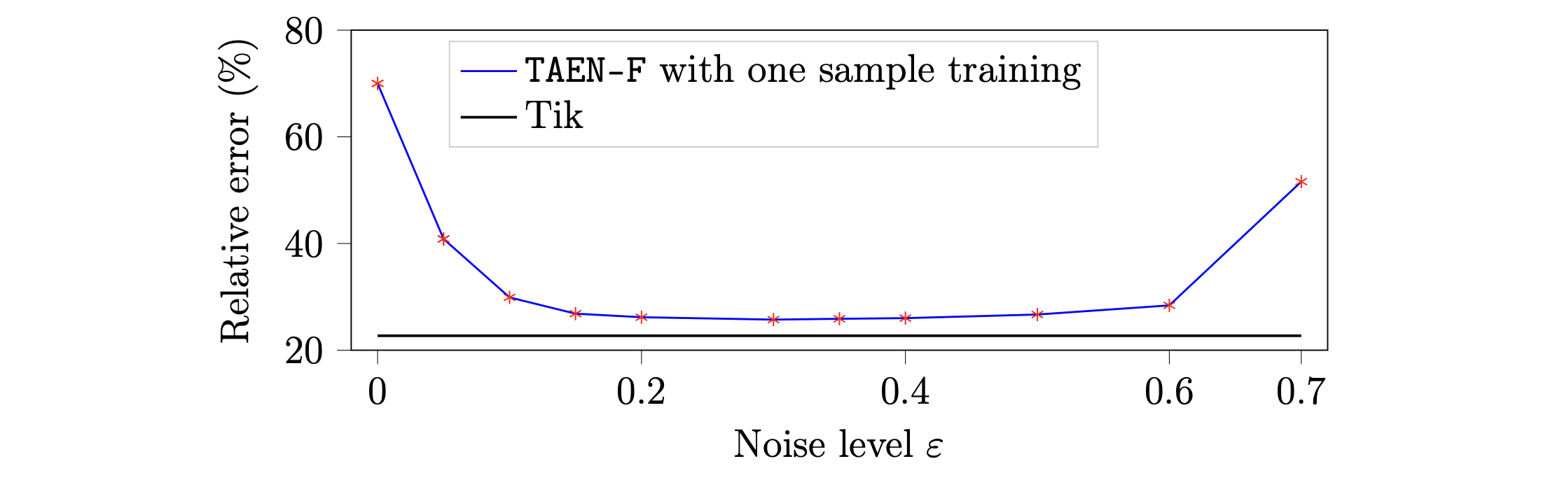
TAENfull robustness to a wide range of noise levels.

A survey of TAENfull trained with one training sample over a wide range of noise levels is shown in Figure 14.

Figure 14: 2D Navier--Stokes equation. Relative error of inverse solution over 500 test samples with different noise levels. As can be seen, the solution accuracy is robust for a wide range of noise from \(\epsilon \in [0.15, 0.5]\). Performance degradation is observed outside of this "optimal" noise level range. At low noise levels, the data randomization process provides insufficient variation to effectively explore the space of unseen test samples, limiting the framework's ability to leverage forward solver constraints. On the other hand, excessive noise levels result in training data becoming statistically indistinguishable, degrading the framework's capacity to learn accurate inverse mappings. These observations are consistent with the theoretical prediction.

TAENfull robustness to arbitrary single-sample.

The robustness of TAENfull to an arbitrary one-training sample is examined. To be more specific, we randomly pick 12 samples out of 100 training sample data sets.

Figure 15: 2D Navier--Stokes equation. Left: Index of \(20\) observational locations. Right: Mean and standard deviation of observation magnitudes of 10000 true observation samples at observational locations. The observation magnitudes of 12 different single-sample training cases. The indices of 20 random observation locations are presented in the left figure. Meanwhile, the mean and standard deviation of observation magnitudes of 10000 true observation samples at corresponding 20 random observation locations and the predicted observation magnitudes from 12 different observation samples are shown in the right figure. From 12 corresponding single-sample training cases, we obtain the mean and standard deviation of the relative error of the inverse solution is \(25.88 \pm 0.19 \%\) (again close to the Tikhonov regularization error). This small variance in relative error metrics demonstrates the TAENfull robustness with respect to an arbitrary individual sample in the single-sample training scenario. In particular, the result shows that the prediction error is similar for any of these 12 individual random samples when used in the TAENfull as the only training sample.

Training Cost and Speedup with Deep Learning Solutions

The training costs for the case of \(n_t = 100\) randomized training samples for heat equation and Navier–Stokes equations are presented in Table 3. It can be observed that the heat equation requires a small amount of training time, about 2 hours, while the corresponding time for the Navier-Stokes equations is about 16 hours. It should be noted that executing the forward map and the backpropagation constitutes the majority of the training cost.

Table 3 also provides information on the computational cost of reconstructing PoIs given an unseen test observation sample and solving for PDE solutions given an unseen PoI sample. Specifically, for inverse solutions, we use the classical Tikhonov (TIK) regularization technique and our proposed deep learning approach TAENfull using the encoder network. In contrast, we use numerical methods and TAENfull decoder for predicting (forward) PDE solutions.

		Heat equation	Navier--Stokes
Training Encoder + Training Decoder (hours)		2	16
Test/Inference (second)	Inverse (Encoder)	$$2.74 \times 10^{-4}$$	$$2.93 \times 10^{-4}$$
	Forward (Decoder)	$$2.86 \times 10^{-4}$$	$$3.06 \times 10^{-4}$$
Numerical solvers (second)	Inverse (Tikhonov)	$$4.36 \times 10^{-2}$$	7.26
	Forward	$$3.01 \times 10^{-2}$$	0.38
Speed up	Inverse	159	24,785
	Forward	105	1,241

Table 3: Training cost and computational speed. The training cost (measured in hours) for the case of \(n_t = 100\) randomized training samples for the heat and Navier--Stokes equations. The computational time (measured in seconds) for forward and inverse solutions using TAENfull and numerical solvers, and the speed-up of TAENfull (the fourth row) relative to numerical solvers using NVIDIA A100 GPUs on Lonestar6 at the Texas Advanced Computing Center (TACC).